ObjectRigidBody
A 3D rigid body which is attached to a 3D rigid body node. The rotation parametrization of the rigid body follows the rotation parametrization of the node. Use Euler parameters in the general case (no singularities) in combination with implicit solvers (GeneralizedAlpha or TrapezoidalIndex2), Tait-Bryan angles for special cases, e.g., rotors where no singularities occur if you rotate about \(x\) or \(z\) axis, or use Lie-group formulation with rotation vector together with explicit solvers. REMARK: Use the class RigidBodyInertia, see Class function: init of exudyn.rigidBodyUtilities to handle inertia, COM and mass.
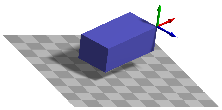
Simpler: mbs.CreateRigidBody adds this item, with what it needs, in one call.
Interface
Python names:
ObjectRigidBodyorRigidBody, andVRigidBodyfor its visualizationNodes it takes: NodeRigidBodyEP, NodeRigidBodyRxyz, NodeRigidBodyRotVecLG
Body markers that can be placed on it: MarkerBodyMass, MarkerBodyPosition, MarkerBodyRigid
Parameters
The parameters of the item; in a dictionary, its type is ‘RigidBody’:
name |
type |
size |
default |
description |
|---|---|---|---|---|
name |
String |
‘’ |
objects’s unique name |
|
mass |
UReal |
0. |
(symbol: \(m\)) mass [SI:kg] of rigid body |
|
inertia |
Vector6D |
6 |
[0.,0.,0., 0.,0.,0.] |
(symbol: \(\LU{b}{\jv_6}\)) inertia components [SI:kgm\(^2\)]: \([J_{xx}, J_{yy}, J_{zz}, J_{yz}, J_{xz}, J_{xy}]\) in body-fixed coordinate system and w.r.t. to the reference point of the body, NOT necessarily w.r.t. to COM; use the class RigidBodyInertia of exudynRigidBodyUtilities.py to handle inertia, COM and mass |
centerOfMass |
Vector3D |
3 |
[0.,0.,0.] |
(symbol: \(\LU{b}{\bv_{COM}}\)) local position of COM relative to the body’s reference point; if the vector of the COM is [0,0,0], the computation will not consider additional terms for the COM and it is faster |
nodeNumber |
NodeIndex |
invalid (-1) |
(symbol: \(n0\)) node number (type NodeIndex) for rigid body node |
|
visualization |
VObjectRigidBody |
parameters for visualization of item |
Renamed parameters, still taken with a DeprecationWarning: physicsMass (deprecated since 1.12.258, removed in 2031): use mass; physicsInertia (deprecated since 1.12.258, removed in 2031): use inertia; physicsCenterOfMass (deprecated since 1.12.258, removed in 2031): use centerOfMass.
Visualization parameters
The parameters of VObjectRigidBody, given as visualization:
name |
type |
size |
default |
description |
|---|---|---|---|---|
show |
Bool |
True |
set true, if item is shown in visualization and false if it is not shown |
|
graphicsDataUserFunction |
ObjectRigidBodyGraphicsDataUserFunction |
0 |
A Python function which returns a bodyGraphicsData object, which is a list of graphics data in a dictionary computed by the user function; the graphics elements need to be defined in the local body coordinates and are transformed by mbs to global coordinates |
|
graphicsData |
BodyGraphicsData |
Structure contains data for body visualization; data is defined in special list / dictionary structure |
Drawing
Drawn as all bodies; its graphicsData in the body frame, and what its graphicsDataUserFunction returns; with a contour plot (contour.rigidBodiesColored) colored by the value at the reference point.
Output variables
Available as OutputVariableType in sensors, Get...Output() and other functions:
output variable |
symbol |
description |
|---|---|---|
Position |
\(\LU{0}{\pv}\cConfig(\pLocB) = \LU{0}{\pRef}\cConfig + \LU{0}{\pRef}\cRef + \LU{0b}{\Rot}\pLocB\) |
global position vector of body-fixed point given by local position vector \(\pLocB\) |
Displacement |
\(\LU{0}{\uv}\cConfig + \LU{0b}{\Rot}\pLocB\) |
global displacement vector of body-fixed point given by local position vector \(\pLocB\) |
Velocity |
\(\LU{0}{\vv}\cConfig(\pLocB) = \LU{0}{\dot\uv}\cConfig + \LU{0b}{\Rot}(\LU{b}{\tomega} \times \pLocB\cConfig)\) |
global velocity vector of body-fixed point given by local position vector \(\pLocB\) |
VelocityLocal |
\(\LU{b}{\vv}\cConfig(\pLocB) = \LU{b0}{\Rot} \LU{0}{\vv}\cConfig(\pLocB)\) |
local (body-fixed) velocity vector of body-fixed point given by local position vector \(\pLocB\) |
RotationMatrix |
\(\mathrm{vec}(\LU{0b}{\Rot})=[A_{00},\,A_{01},\,A_{02},\,A_{10},\,\ldots,\,A_{21},\,A_{22}]\cConfig\tp\) |
vector with 9 components of the rotation matrix (row-major format) |
Rotation |
vector with 3 components of the Euler angles in xyz-sequence (R=RxRyRz), recomputed from rotation matrix |
|
AngularVelocity |
\(\LU{0}{\tomega}\cConfig\) |
global 3D angular velocity vector of body |
AngularVelocityLocal |
\(\LU{b}{\tomega}\cConfig\) |
local (body-fixed) 3D angular velocity vector of body |
Acceleration |
\(\LU{0}{\av}\cConfig(\pLocB) = \LU{0}{\ddot\uv} + \LU{0}{\talpha} \times (\LU{0b}{\Rot} \pLocB) + \LU{0}{\tomega} \times ( \LU{0}{\tomega} \times(\LU{0b}{\Rot} \pLocB))\) |
global acceleration vector of body-fixed point given by local position vector \(\pLocB\) |
AccelerationLocal |
\(\LU{b}{\av}\cConfig(\pLocB) = \LU{b0}{\Rot} \LU{0}{\av}\cConfig(\pLocB)\) |
local (body-fixed) acceleration vector of body-fixed point given by local position vector \(\pLocB\) |
AngularAcceleration |
\(\LU{0}{\talpha}\cConfig\) |
angular acceleration vector of body |
AngularAccelerationLocal |
\(\LU{b}{\talpha}\cConfig = \LU{b0}{\Rot} \LU{0}{\talpha}\cConfig\) |
local angular acceleration vector of body |
KineticEnergy |
\(T = \frac{1}{2} m\, \LU{0}{\vv}\tp\LU{0}{\vv} + m\, \LU{0}{\vv}\tp (\LU{0}{\tomega} \times \LU{0b}{\Rot}\LU{b}{\bv_{COM}}) + \frac{1}{2} \LU{b}{\tomega}\tp \LU{b}{\Jm} \LU{b}{\tomega}\) |
kinetic energy of the body, with the velocity \(\LU{0}{\vv}\) of its reference point and the inertia w.r.t. it; localPosition must be \([0,0,0]\) |
PotentialEnergy |
\(V = 0\) |
the body has no elastic energy; gravity and other loads are not part of it (see exudyn.advancedUtilities.LoadPotentialEnergy) - the value stays the same when a body gets a built-in gravity; localPosition must be \([0,0,0]\) |
Detailed description
Definition of quantities
intermediate variables |
symbol |
description |
|---|---|---|
inertia tensor |
\(\LU{b}{\Jm} = \LU{b}{\mr{J_{xx}}{J_{xy}}{J_{xz}} {J_{xy}}{J_{yy}}{J_{yz}} {J_{xz}}{J_{yz}}{J_{zz}}}\) |
symmetric inertia tensor, based on components of \(\LU{b}{\jv_6}\), in body-fixed (local) coordinates and w.r.t. body’s reference point |
reference coordinates |
\(\qv\cRef = [\pRef\tp\cRef,\,\tpsi\tp\cRef]\tp\) |
defines reference configuration, DIFFERENT meaning from body’s reference point! |
(relative) current coordinates |
\(\qv\cCur = [\pRef\tp\cCur,\,\tpsi\tp\cCur]\tp\) |
unknowns in solver; relative to the reference coordinates; current coordinates at initial configuration = initial coordinates \(\qv\cIni\) |
current velocity coordinates |
\(\dot \qv\cCur = [\vv\tp\cCur,\,\dot \tpsi\tp\cCur]\tp = [\dot \pv\tp\cCur,\,\dot \ttheta\tp\cCur]\tp\) |
current velocity coordinates |
body’s reference point |
\(\pRefG\cConfig + \pRefG\cRef = \LU{0}{\pv}(n_0)\cConfig\) |
position of body’s reference point provided by node \(n_0\) in any configuration except for reference; if \(\LU{b}{\bv_{COM}}==[0,\;0,\;0]\tp\), this position becomes equal to the COM position |
reference body’s reference point |
\(\pRefG\cRef = \LU{0}{\pv}(n_0)\cRef\) |
position of body’s reference point in reference configuration |
body’s reference point displacement |
\(\LU{0}{\uv}\cConfig = \pRefG\cConfig = [q_0,\;q_1,\;q_2]\cConfig\tp = \LU{0}{\uv}(n_0)\cConfig\) |
displacement of body’s reference point which is provided by node \(n_0\) in any configuration |
body’s reference point velocity |
\(\LU{0}{\vv}\cConfig = \dot \pRefG\cConfig = [\dot q_0,\;\dot q_1,\;\dot q_2]\cConfig\tp = \LU{0}{\vv}(n_0)\cConfig\) |
velocity of body’s reference point which is provided by node \(n_0\) in any configuration |
body’s reference point acceleration |
\(\LU{0}{\av}\cConfig = [\ddot q_0,\;\ddot q_1,\;\ddot q_2]\cConfig\tp\) |
acceleration of body’s reference point which is provided by node \(n_0\) in any configuration |
rotation coordinates |
\(\ttheta_{\mathrm{config}} = \tpsi(n_0)\cRef + \tpsi(n_0)\cConfig\) |
(total) rotation parameters of body as provided by node \(n_0\) in any configuration |
rotation parameters |
\(\ttheta_{\mathrm{config}} = \tpsi(n_0)\cRef + \tpsi(n_0)\cConfig\) |
(total) rotation parameters of body as provided by node \(n_0\) in any configuration |
body rotation matrix |
\(\LU{0b}{\Rot}\cConfig = \LU{0b}{\Rot}(n_0)\cConfig\) |
rotation matrix which transforms local to global coordinates as given by node |
local position |
\(\pLocB = [\LU{b}{b_0},\,\LU{b}{b_1},\,\LU{b}{b_2}]\tp\) |
local position as used by markers or sensors |
angular velocity |
\(\LU{0}{\tomega}\cConfig = \LU{0}{[\omega_0(n_0),\,\omega_1(n_0),\,\omega_2(n_0)]}\cConfig\tp\) |
global angular velocity of body as provided by node \(n_0\) in any configuration |
local angular velocity |
\(\LU{b}{\tomega}\cConfig\) |
local angular velocity of body as provided by node \(n_0\) in any configuration |
body angular acceleration |
\(\LU{0}{\talpha}\cConfig = \LU{0}{\dot \tomega}\cConfig\) |
angular acceleratoin of body as provided by node \(n_0\) in any configuration |
applied forces |
\(\LU{0}{\fv}_a = [f_0,\;f_1,\;f_2]\tp\) |
calculated from loads, connectors, … |
applied torques |
\(\LU{0}{\ttau}_a = [\tau_0,\;\tau_1,\;\tau_2]\tp\) |
calculated from loads, connectors, … |
constraint reaction forces |
\(\LU{0}{\fv}_\lambda = [f_{\lambda 0},\;f_{\lambda 1},\;f_{\lambda 2}]\tp\) |
calculated from joints or constraint) |
constraint reaction torques |
\(\LU{0}{\ttau}_\lambda = [\tau_{\lambda 0},\;\tau_{\lambda 1},\;\tau_{\lambda 2}]\tp\) |
calculated from joints or constraints |
Rotation parametrization
The equations of motion of the rigid body build upon a specific parameterization of the rigid body coordinates.
Rigid body coordinates are defined by the underlying node given by nodeNumber \(n0\).
Appropriate nodes are
NodeRigidBodyEP(Euler parameters)NodeRigidBodyRxyz(Euler angles / Tait Bryan angles)NodeRigidBodyRotVecLG(Rotation vector with Lie group integration option)
Note that all operations for rotation parameters, such as the computation of the rotation matrix, must be performed with the rotation parameters \(\ttheta\), see table above, which are the sum of reference and current coordinates.
The angular velocity in body-fixed coordinates is related to the rotation parameters by means of a matrix \(\LU{b}{\Gm_{rp}}\),
and is specific for any rotation parametrization \(rp\). The angular velocity in global coordinates is related to the rotation parameters by means of a matrix \(\LU{0}{\Gm_{rp}}\),
The local angular accelerations follow as
remember that derivatives for angular velocities can also be done in the local frame. In case of Euler parameters and the Lie-group rotation vector we find that \(\LU{b}{\dot \Gm_{rp}} \dot \ttheta = \Null\).
Equations of motion for COM
The equations of motion for a rigid body, the so-called Newton-Euler equations, can be written for the special case of the reference point \(=\) COM and split for translations and rotations, using a coordinate-free notation,
with the \(3\times 3\) unit matrix \(\ImThree\) and forces \(\fv\) resp. torques \(\ttau\) as discribed in the table above. A change of the reference point, using the vector \(\bv_{COM}\) from the body’s reference point \(\pv\) to the COM position, is simple by replacing COM accelerations using the common relation known from Euler
which is inserted into the first line of (50). Additionally, the second line of (50) (second Euler equation related to rate of angular momentum) is rewritten for an arbitrary reference point, \(\bv_{COM}\) denoting the vector from the body reference point to COM, using the well known relation
Equations of motion for arbitrary reference point
This immediately leads to the equations of motion for the rigid body with respect to an arbitrary reference point (\(\neq\) COM), see e.g. woernle2016(page 258ff.), which have the general coordinate-free form
in which \(\Jm\) is the inertia tensor w.r.t. the chosen reference point (which has local coordinates \(\LU{b}{[0,0,0]\tp}\)). (51) can be written in the global frame (0),
Expressing the translational part (first line) of (52) in the global frame (0), using local coordinates (b) for quantities that are constant in the body-fixed frame, \(\LU{b}{\Jm}\) and \(\LU{b}{\bv_{COM}}\), thus expressing also the angular velocity \(\LU{b}{\tomega}\) in the body-fixed frame, applying (47) and (49), and using the relations
we obtain
with constraint reaction forces \(\fv_{\theta,\lambda}\) for the rotation parameters. Note that the last line has been pre-multiplied with \(\LU{b}{\Gm_{rp}\tp}\) (in order to make the mass matrix symmetric) and that \(\LU{b}{\dot \Gm_{rp}} \dot \ttheta = \Null\) in case of Euler parameters and the Lie-group rotation vector .
Euler parameters
In case of Euler parameters, a constraint equation is automatically added, reading for the index 3 case
and for the index 2 case
Given a Lagrange parameter (algebraic variable) \(\lambda_\theta\) related to the Euler parameter constraint (54), the constraint reaction forces in (53) then read
Marker interfaces
A local position \(\pLocB\) of the body moves with the velocity \(\LU{0}{\vv} + \LU{0b}{\Rot} (\LU{b}{\tomega} \times \pLocB)\), which gives, with the velocity transformations of the node, the position and rotation Jacobians
with \(\LU{b}{\tilde \pv}_{\mathrm{loc}}\) the skew-symmetric matrix of \(\pLocB\); a force at the local position then acts on the rotation coordinates with the moment it has about the reference point. The mass-weighted Jacobian of a mass-proportional load is \(m\) times the position Jacobian of the center of mass.
Userfunction: graphicsDataUserFunction(mbs, itemNumber)
A user function, which is called by the visualization thread in order to draw user-defined objects.
The function can be used to generate any BodyGraphicsData, see Section GraphicsData.
Use exudyn.graphics functions, see Section Module: graphics, to create more complicated objects.
Note that graphicsDataUserFunction needs to copy lots of data and is therefore
inefficient and only designed to enable simpler tests, but not large scale problems.
For an example for graphicsDataUserFunction see ObjectGround, ObjectGround.
arguments / return |
type or size |
description |
|---|---|---|
|
MainSystem |
provides reference to mbs, which can be used in user function to access all data of the object |
|
Index |
integer number of the object in mbs, allowing easy access |
return value |
BodyGraphicsData |
list of |
Mini example
#a rigid body thrown with a spin about a principal axis, under gravity
inertia = InertiaCuboid(density=1000, sideLengths=[0.4,0.2,0.1])
node = mbs.AddNode(NodeRigidBodyEP(referenceCoordinates=[0.5,0.2,0]+eulerParameters0,
                                   initialVelocities=[0,0,5]+list(AngularVelocity2EulerParameters_t([0,0,1], eulerParameters0))))
body = mbs.AddObject(ObjectRigidBody(nodeNumber=node, mass=inertia.Mass(),
                                     inertia=inertia.GetInertia6D()))
mMass = mbs.AddMarker(MarkerBodyMass(bodyNumber=body))
mbs.AddLoad(LoadMassProportional(markerNumber=mMass, loadVector=[0,0,-9.81]))

mbs.Assemble()
mbs.SolveDynamic()

#z = v0*t - g/2*t^2, and the angle about z is omega*t, at t=1
p = mbs.GetNodeOutput(node, exu.OutputVariableType.Position)
angle = mbs.GetNodeOutput(node, exu.OutputVariableType.Rotation)[2]
exu.sys['testResult'] = p[2] + angle #0.095 + 1
Examples (Ex) and TestModels (TM) that show this item, with weblink to github: tutorialRigidBody.py (Ex), tutorialRigidBodyCreate.py (Ex), fourBarMechanism3D.py (Ex)