Flexible body – FFRF tutorial
The following tutorial includes flexible bodies, using the floating frame of reference formulation (FFRF), including Netgen and NGsolve for mesh and finite element data generation and uses modal reduction for simulation. The tutorial will set up a body with Hurty-Craig-Bampton modes, giving a simple flexible pendulum meshed hinged with a revolute joint.

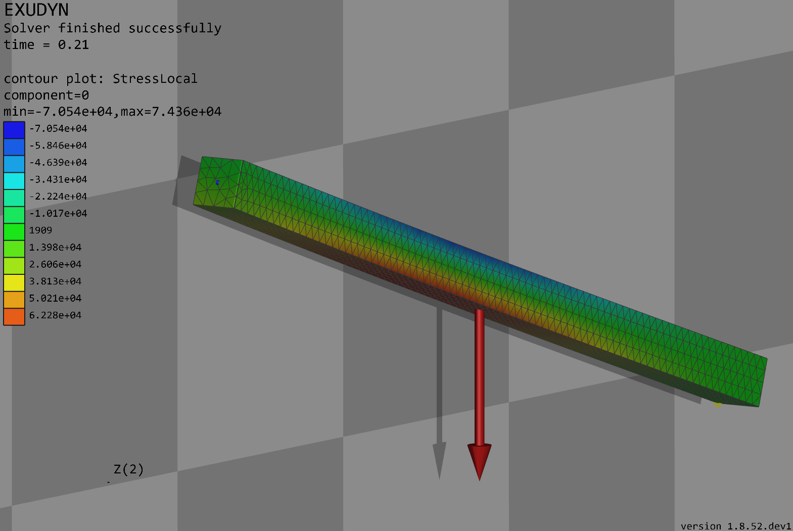
Fig. 13 Screen shot of pendulum modeled with floating frame of reference formulation, using HCB modes, and meshed with Netgen.
We import the exudyn library, utilities, and other necessary modules:
import exudyn as exu
from exudyn.utilities import *  # includes itemInterface and rigidBodyUtilities
import exudyn.graphics as graphics  # only import if it does not conflict
from exudyn.FEM import *
import numpy as np
import time
import ngsolve as ngs
from netgen.meshing import *
from netgen.csg import *
Next, we need a SystemContainer, which contains all computable systems and adds a new MainSystem mbs:
SC = exu.SystemContainer()
mbs = SC.AddSystem()
Define the parameters and setup the Netgen mesh, using Netgen’s CSG geometry. We create a simple brick in order to simplify the application of boundary interfaces and joints:
useGraphics = True
fileName = 'testData/netgenBrick'  # for load/save of FEM data

a = 0.025  # height/width of beam
b = a
h = 0.5 * a
L = 1     # Length of beam
nModes = 8

rho = 1000
Emodulus = 1e7 * 10
nu = 0.3
meshCreated = False
meshOrder = 1  # use order 2 for higher accuracy, but more unknowns

geo = CSGeometry()
block = OrthoBrick(Pnt(0, -a, -b), Pnt(L, a, b))
geo.Add(block)
mesh = ngs.Mesh(geo.GenerateMesh(maxh=h))
mesh.Curve(1)
When creating the geometry and mesh, we sometimes would like to verify that with Netgen’s GUI.
In Jupyter, this works smoother with webgui_jupyter_widgets – see the Netgen documention. Here we use a simple loop, which has to set True if visualization shall run:
if False:  # set this to true, if you want to visualize the mesh inside netgen/ngsolve
    import netgen.gui
    ngs.Draw(mesh)
    for i in range(10000000):
        netgen.Redraw()  # this makes the window interactive
        time.sleep(0.05)
Use the FEM interface to import the FEM model and create the FFRF reduced-order data stored in fem. Note that on importing the FEM structure from NGsolve (the FEM-module and solver of Netgen), we have to specify the mechanical properties related to the mesh:
fem = FEMinterface()
[bfM, bfK, fes] = fem.ImportMeshFromNGsolve(mesh, density=rho,
                                            youngsModulus=Emodulus,
                                            poissonsRatio=nu,
                                            meshOrder=meshOrder)
We could now just compute eigenmodes of the free bodies. However, as mentioned in the theory part, they do not respect boundary conditions and lead to low accuracy. Therefore, we use Hurty-Craig-Bampton modes.
For them, we have to define boundary interfaces given as lists of node numbers as well as weights.
We can use convenient functions from the FEMinterface class to retrieve nodes from planar or cylindrical surfaces (or we may define them in the finite element model ourselves):
pLeft = [0, -a, -b]
pRight = [L, -a, -b]
nTip = fem.GetNodeAtPoint(pRight) #for sensor
nodesLeftPlane = fem.GetNodesInPlane(pLeft, [-1, 0, 0])
weightsLeftPlane = fem.GetNodeWeightsFromSurfaceAreas(nodesLeftPlane)
nodesRightPlane = fem.GetNodesInPlane(pRight, [-1, 0, 0])
weightsRightPlane = fem.GetNodeWeightsFromSurfaceAreas(nodesRightPlane)
We define a list of boundaries, which are then passed to the function which computes modes. Note that by default the first boundary modes are eliminated as they are fixed to the reference frame of the FFRF object:
boundaryList = [nodesLeftPlane]

print("nNodes=", fem.NumberOfNodes())
print("compute HCB modes... ")
start_time = time.time()
fem.ComputeHurtyCraigBamptonModes(boundaryNodesList=boundaryList,
                                  nEigenModes=nModes,
                                  useSparseSolver=True,
                                  computationMode=HCBstaticModeSelection.RBE2)
print("HCB modes needed
Compute stress modes for postprocessing, which is not needed for simulation, but useful for postprocessing:
if True:
    mat = KirchhoffMaterial(Emodulus, nu, rho)
    varType = exu.OutputVariableType.StressLocal
    print("ComputePostProcessingModes ... (may take a while)")
    start_time = time.time()
    fem.ComputePostProcessingModesNGsolve(fes, material=mat,
                                          outputVariableType=varType)
    print("   ... needed
    SC.visualizationSettings.contour.reduceRange = False
    SC.visualizationSettings.contour.outputVariable = varType
    SC.visualizationSettings.contour.outputVariableComponent = 0  # x-component
else:
    SC.visualizationSettings.contour.outputVariable = exu.OutputVariableType.DisplacementLocal
    SC.visualizationSettings.contour.outputVariableComponent = 1
Having all data prepared now, we create the CMS element which is an object added then to mbs:
print("create CMS element ...")
cms = ObjectFFRFreducedOrderInterface(fem)
objFFRF = cms.AddObjectFFRFreducedOrder(mbs, positionRef=[0, 0, 0],
                                        initialVelocity=[0, 0, 0],
                                        initialAngularVelocity=[0, 0, 0],
                                        gravity=[0, -9.81, 0],
                                        color=[0.1, 0.9, 0.1, 1.])
Add markers and revolute joint, using a superelement marker:
nodeDrawSize = 0.0025  # for joint drawing

mRB = mbs.AddMarker(MarkerNodeRigid(nodeNumber=objFFRF['nRigidBody']))
oGround = mbs.AddObject(ObjectGround(referencePosition=[0, 0, 0]))
leftMidPoint = [0, 0, 0]
mGround = mbs.AddMarker(MarkerBodyRigid(bodyNumber=oGround, localPosition=leftMidPoint))
mLeft = mbs.AddMarker(MarkerSuperElementRigid(bodyNumber=objFFRF['oFFRFreducedOrder'],
                                              meshNodeNumbers=np.array(nodesLeftPlane),
                                              weightingFactors=weightsLeftPlane))
mbs.AddObject(GenericJoint(markerNumbers=[mGround, mLeft],
                           constrainedAxes=[1, 1, 1, 1, 1, 1 * 0],
                           visualization=VGenericJoint(axesRadius=0.1 * a, axesLength=0.1 * a)))
Note that the marker is using weights, which are needed to compute accurate average (midpoint) positions from the non-uniform triangular surface mesh.
Now we finally add a sensor and assemble the system:
fileDir = 'solution/'
sensTipDispl = mbs.AddSensor(SensorSuperElement(bodyNumber=objFFRF['oFFRFreducedOrder'],
                                                meshNodeNumber=nTip,
                                                fileName=fileDir + 'nMidDisplacementCMS' + str(nModes) + 'Test.txt',
                                                outputVariableType=exu.OutputVariableType.Displacement))

mbs.Assemble()
Set simulation settings and run the simulation:
simulationSettings = exu.SimulationSettings()

SC.visualizationSettings.nodes.defaultSize = nodeDrawSize
SC.visualizationSettings.nodes.drawNodesAsPoint = False
SC.visualizationSettings.connectors.defaultSize = 2 * nodeDrawSize
SC.visualizationSettings.nodes.show = False
SC.visualizationSettings.sensors.show = True
SC.visualizationSettings.sensors.defaultSize = 0.01
SC.visualizationSettings.markers.show = False
SC.visualizationSettings.loads.drawSimplified = False

h = 1e-3
tEnd = 4

simulationSettings.timeIntegration.numberOfSteps = int(tEnd / h)
simulationSettings.timeIntegration.endTime = tEnd
simulationSettings.timeIntegration.verboseMode = 1
simulationSettings.timeIntegration.newton.useModifiedNewton = True
simulationSettings.solutionSettings.sensorsWritePeriod = h
simulationSettings.timeIntegration.generalizedAlpha.spectralRadius = 0.8
simulationSettings.displayComputationTime = True

mbs.SolveDynamic(simulationSettings=simulationSettings)

uTip = mbs.GetSensorValues(sensTipDispl)[1]
print("nModes=", nModes, ", tip displacement=", uTip)

mbs.SolutionViewer()
When the solution viewer starts, it should show the stresses in a flexible swinging pendulum, see Fig. 13.
NOTE: this tutorial has been mostly created with ChatGPT-4, and curated hereafter!