Items: Nodes, Objects, Loads, Markers, Sensors, …
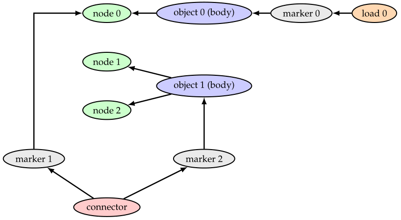
In this section, the most important part of Exudyn are provided. An overview of the interaction of the items is given in Fig. 4

Fig. 4 Interaction of items in a multibody system
Note that both, bodies and connectors (including constraints) are – computational – objects. The arrows indicate, that, e.g., object 1 has node 1 and node 2 (indexes) and that marker 0 is attached to object 0, while load 0 uses marker 0 to apply the load. Sensors could additionally be attached to certain items.
Nodes
Nodes provide the coordinates (and the degrees of freedom) to the system. They have no mass, stiffness or whatsoever assigned.
Without nodes, the system has no unknown coordinates.
Adding a node provides (for the system unknown) coordinates. In addition we also need equations for every nodal coordinate – otherwise the system cannot be computed (NOTE: this is currently not checked by the preprocessor).
In general, adding nodes and objects (e.g., to represent rigid bodies), leads to a redundant coordinate formulation.
In order to determine the degree of freedom, you may use the Grübler-Kutzbach criterion. This can also be done numerically, using the function ComputeSystemDegreeOfFreedom, see the module exudyn.solver.
Furthermore, minimal coordinates can be used for open tree systems, using ObjectKinematicTree.
Objects
Objects are ‘computational objects’ and they provide equations to your system. Objects often provide derivatives and have measurable quantities (e.g. displacement) and they provide access, which can be used to apply, e.g., forces. Some of this functionality is only available in C++, but not in Python.
Objects can be a:
general object (e.g. a controller, user defined object, …; no example yet)
body: has a mass or mass distribution; markers can be placed on bodies; loads can be applied; constraints can be attached via markers; bodies can be:
ground object: has no nodes
simple body: has one node (e.g. mass point, rigid body)
finite element and more complicated body (e.g. FFRF-object): has more than one node
connector: uses markers to connect nodes and/or bodies; adds additional terms to system equations either based on stiffness/damping or with constraints (and Lagrange multipliers). Possible connectors:
algebraic constraint (e.g. constrain two coordinates: \(q_1 = q_2\))
classical joint
spring-damper or penalty constraint
Markers
Markers are interfaces between objects/nodes and constraints/loads. A constraint (which is also an object) or load cannot act directly on a node or object without a marker. As a benefit, the constraint or load does not need to know whether it is applied, e.g., to a node or to a local position of a body.
Typical situations are:
Node – Marker – Load
Node – Marker – Constraint (object)
Body(object) – Marker – Load
Body1 – Marker1 – Joint(object) – Marker2 – Body2
Loads
Loads are used to apply forces and torques to the system. The load values are static values. However, you can use Python functionality to modify loads either by linearly increasing them during static computation or by using the ‘mbs.SetPreStepUserFunction(…)’ structure in order to modify loads in every integration step depending on time or on measured quantities (thus, creating a controller).
Sensors
Sensors are only used to measure output variables (values) in order to simpler generate the requested output quantities. They have a very weak influence on the system, because they are only evaluated after certain solver steps as requested by the user.
Reference coordinates and displacements
Nodes usually have separated reference and initial quantities.
Here, referenceCoordinates are the coordinates for which the system is defined upon creation.
Reference coordinates are needed, e.g., for definition of joints and for the reference configuration of finite elements. In many cases it marks the undeformed configuration (e.g., with finite elements), but not, e.g., for ObjectConnectorSpringDamper, which has its own reference length.
Initial displacement (or rotation) values are provided separately, in order to start a system from a configuration different from the reference configuration.
As an example, the initial configuration of a NodePoint is given by referenceCoordinates + initialCoordinates, while the initial state of a dynamic system additionally needs initialVelocities.
See also Section Reference and current coordinates!
Note that commonly the OutputVariableType Coordinates returns coordinates without reference values, which are usually displacements (or changes in the rotation parameters), which is required if you are interested, e.g., in motion of finite element nodes.
In contrast the OutputVariableType CoordinatesTotal returns (Since Exudyn1.9.25) the sum of reference and displacement (or rotation) coordinates for any configuration (e.g., current, initial or visualization).