ObjectContactSphereSphere

A simple contact connector between two spheres, using various contact models and the option for contact of sphere inside hollow sphere (marker1). The connector implements at least the same functionality as in GeneralContact and is intended for simple setups and for testing, while GeneralContact is much more efficient due to parallelization approaches and efficient contact search.

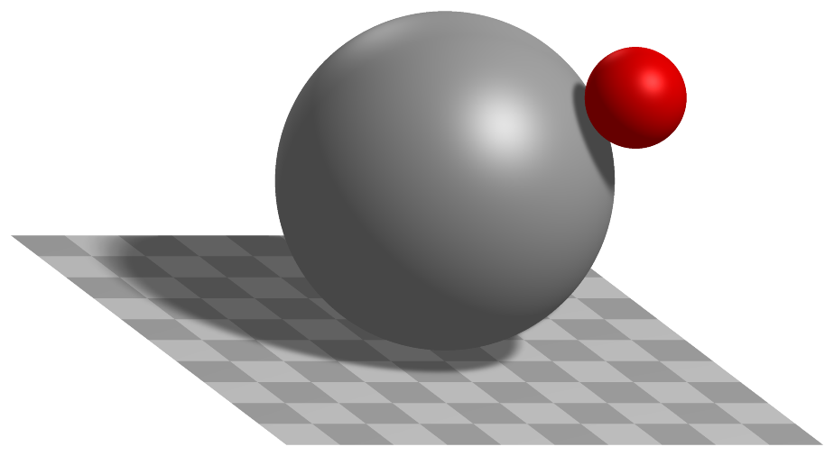
Authors: Gerstmayr Johannes, Weyrer Sebastian

Simpler: mbs.CreateSphereSphereContact adds this item, with what it needs, in one call.

Interface

• Nodes it takes: NodeGenericData

• Markers it acts on: those providing Position (and Orientation if dynamicFriction is not zero): MarkerBodyPosition, MarkerBodyRigid, MarkerNodePosition, MarkerNodeRigid, MarkerSuperElementPosition, MarkerSuperElementRigid, MarkerKinematicTreeRigid

Parameters

The parameters of the item; in a dictionary, its type is ‘ContactSphereSphere’:

name	type	size	default	description
name	String		‘’	constraints’s unique name
markerNumbers	ArrayMarkerIndex	2	[ invalid (-1), invalid (-1) ]	(symbol: \([m0,m1]\tp\)) list of markers representing centers of spheres, used in connector
nodeNumber	NodeIndex		invalid (-1)	(symbol: \(n_d\)) node number of a NodeGenericData with numberOfDataCoordinates = 4 dataCoordinates, needed for discontinuous iteration (friction and contact); data variables contain values from last PostNewton iteration: data[0] is the gap, data[1] is the norm of the tangential velocity (and thus contains information if it is stick or slip); data[2] is the impact velocity; data[3] is the plastic overlap of the Edinburgh Adhesive Elasto-Plastic Model, initialized usually with 0 and set back to 0 in case that spheres have been separated.
spheresRadii	Vector2D	2	[-1.,-1.]	(symbol: \([r_0,r_1]\tp\)) list containing radius of sphere 0 and radius of sphere 1 [SI:m].
isHollowSphere1	Bool		False	flag, which determines, if sphere attached to marker 1 (radius 1) is a hollow sphere.
dynamicFriction	UReal		0.	(symbol: \(\mu_d\)) dynamic friction coefficient for friction model, see StribeckFunction in exudyn.physics, Module: physics
frictionProportionalZone	UReal		0.001	(symbol: \(v_{reg}\)) limit velocity [m/s] up to which the friction is proportional to velocity (for regularization / avoid numerical oscillations), see StribeckFunction in exudyn.physics (named regVel there!), Module: physics
contactStiffness	UReal		0.	(symbol: \(k_c\)) normal contact stiffness [SI:N/m] (units in case that \(n_\mathrm{exp}=1\))
contactDamping	UReal		0.	(symbol: \(d_c\)) linear normal contact damping [SI:N/(m s)]; this damping should be used (!=0) if the restitution coefficient is < 1, as it changes its behavior.
contactStiffnessExponent	PReal		1.	(symbol: \(n_\mathrm{exp}\)) exponent in normal contact model [SI:1]
constantPullOffForce	UReal		0.	(symbol: \(f_\mathrm{adh}\)) constant adhesion force [SI:N]; Edinburgh Adhesive Elasto-Plastic Model
contactPlasticityRatio	UReal		0.	(symbol: \(\lambda_\mathrm{P}\)) ratio of contact stiffness for first loading and unloading/reloading [SI:1]; Edinburgh Adhesive Elasto-Plastic Model; \(\lambda_\mathrm{P}=1-k_c/K2\), which gives the contact stiffness for unloading/reloading \(K2 = k_c/(1-\lambda_\mathrm{P})\); set to 0 in order to fully deactivate Edinburgh Adhesive Elasto-Plastic Model model
adhesionCoefficient	UReal		0.	(symbol: \(k_\mathrm{adh}\)) coefficient for adhesion [SI:N/m] (units in case that \(n_\mathrm{adh}=1\)); Edinburgh Adhesive Elasto-Plastic Model; set to 0 to deactivate adhesion model
adhesionExponent	UReal		1.	(symbol: \(n_\mathrm{adh}\)) exponent for adhesion coefficient [SI:1]; Edinburgh Adhesive Elasto-Plastic Model
restitutionCoefficient	PReal		1.	(symbol: \(e_\mathrm{res}\)) coefficient of restitution [SI:1]; used in particular for impact mechanics; different models available within parameter impactModel; the coefficient must be > 0, but can become arbitrarily small to emulate plastic impact (however very small values may lead to numerical problems)
minimumImpactVelocity	UReal		0.	(symbol: \(\dot\delta_\mathrm{-,min}\)) minimal impact velocity for coefficient of restitution [SI:1]; this value adds a lower bound for impact velocities for calculation of viscous impact force; it can be used to apply a larger damping behavior for low impact velocities (or permanent contact)
impactModel	UInt		0	(symbol: \(m_\mathrm{impact}\)) number of impact model: 0) linear model (only linear damping is used); 1) Hunt-Crossley model; 2) Gonthier/EtAl-Carvalho/Martins mixed model; model 2 is much more accurate regarding the coefficient of restitution, in the full range [0,1] except for 0; NOTE: in all models, the linear contactDamping is added, if not set to zero!
activeConnector	Bool		True	flag, which determines, if the connector is active; used to deactivate (temporarily) a connector or constraint
visualization	VObjectContactSphereSphere			parameters for visualization of item

Visualization parameters

The parameters of VObjectContactSphereSphere, given as visualization:

name	type	size	default	description
show	Bool		False	set true, if item is shown in visualization and false if it is not shown; draws spheres by given radii
color	Float4	4	[0.7,0.7,0.7,1.]	RGBA connector color; if R==-1, use default color

Drawing

Drawn as all connectors; the two spheres with contact.showSpheres, in contact.colorSpheres.

Settings beyond those of all connectors: contact.colorSpheres, contact.showSpheres, contact.tilingSpheres.

Output variables

Available as OutputVariableType in sensors, Get...Output() and other functions:

output variable	symbol	description
Position		contact center point (also given for positive gap, when no contact occurs)
Displacement		global displacement vector between the two spheres midpoints
DisplacementLocal		1D Vector, containing only gap
Velocity		global relative velocity between the two spheres midpoints
Force		global contact force vector
Director1		contains normalized vector from marker 0 to marker 1
Torque		global torque due to friction on marker 0; to obetain torque on marker 1, multiply the torque with the factor \(\frac{r_1+g/2}{r_0+g/2}\)

Detailed description

Definition of quantities

intermediate variables	symbol	description
marker m0 position	\(\LU{0}{\pv}_{m0}\)	global position of sphere 0 center as provided by marker m0
marker m0 orientation	\(\LU{0,m0}{\Rot}\)	current rotation matrix provided by marker m0
marker m1 position	\(\LU{0}{\pv}_{m1}\)	global position of sphere 1 center as provided by marker m1
marker m1 orientation	\(\LU{0,m1}{\Rot}\)	current rotation matrix provided by marker m1
data coordinates	\(\xv=[x_0,\,x_1,\,x_2,\,x_3]\tp\)	hold the current gap (0), the (norm of the) tangential velocity (1), the impact velocity (2), and the plastic deformation (3) of the adhesion model
marker m0 velocity	\(\LU{0}{\vv}_{m0}\)	current global velocity which is provided by marker m0
marker m1 velocity	\(\LU{0}{\vv}_{m1}\)	current global velocity which is provided by marker m1
marker m0 angular velocity	\(\LU{0}{\tomega}_{m0}\)	current angular velocity vector provided by marker m0
marker m1 angular velocity	\(\LU{0}{\tomega}_{m1}\)	current angular velocity vector provided by marker m1

Connector forces

This section outlines the computation of the forces acting on the two spheres when they are in contact with each other. Two types of forces can act on the spheres due to the connector:

• normal force computed according to the chosen impact model \(m_\mathrm{impact}\) and with contact damping if \(d_c\neq0\); this type of force does not create a torque acting on the spheres.

• tangential force due to a regularized friction law to model dry friction between the spheres; this type of force creates a torque acting on the spheres and is computed independently of the chosen impact model if \(\mu_d\neq0\) is set. Note that in the implemented model, rolling deformations are not considered, i.e. the friction is only a function of the relative tangential velocity between the spheres at the contact point.

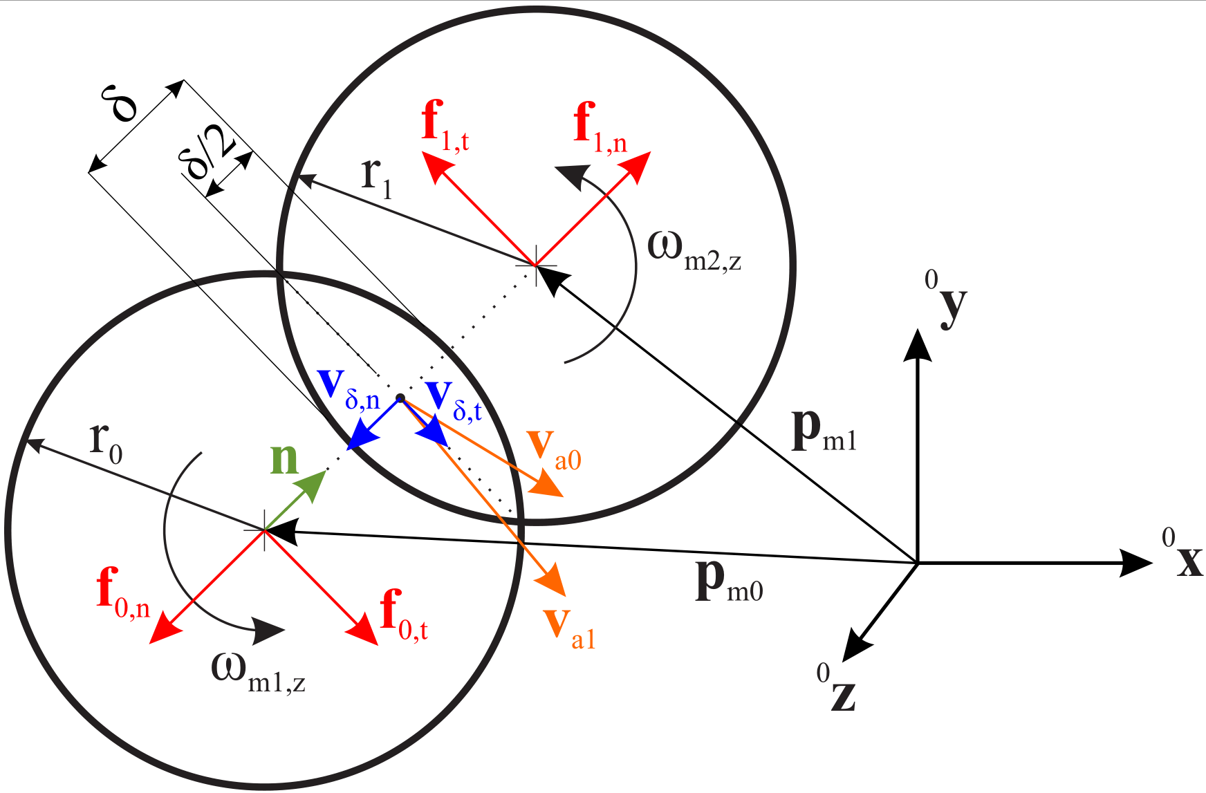
Fig. 43 Two spheres that are in contact, showing a force on marker 1 in normal direction due to overlap; forces on marker 0 act in opposite direction.

Calculations reflect the case for outer contact of two spheres using \(h_1=1\). In case that isHollowSphere1=True, we set \(h_1=-1\) while the remaining formulas are unchanged. In Fig. 43 the sphere sphere and in Fig. 44 the sphere hollowsphere contact case are shown.

For the following, the gap \(g\) between the two spheres is computed as

\[ g = h_1 || \LU{0}{\pv}_{m1} - \LU{0}{\pv}_{m0} || - (r_0 + h_1 r_1) \]

and the overlap \(\delta\) is the negated gap: \(\delta=-g\). In the contact case, the overlap \(\delta\) is positive. If the first sphere is a hollow sphere, the gap consequently reads

\[ g = r_1 - r_0 - || \LU{0}{\pv}_{m1} - \LU{0}{\pv}_{m0} || \, , \]

such that if sphere 0 is in contact with the inner side of sphere 1, i.e. \(|| \LU{0}{\pv}_{m1} - \LU{0}{\pv}_{m0} ||\geq(r_1-r_0)\) holds, the gap is negative and the overlap \(\delta\) is positive. The normal vector \(\LU{0}{\nv}\) always points from marker 0 to the contact point:

\[ \LU{0}{\nv} = h_1 \frac{\LU{0}{\pv}_{m1} - \LU{0}{\pv}_{m0}}{|| \LU{0}{\pv}_{m1} - \LU{0}{\pv}_{m0} ||} \, . \]

In the case of sphere-sphere contact, \(\LU{0}{\nv}\) points from marker 0 to marker 1, and in the case of sphere-hollowsphere contact, \(\LU{0}{\nv}\) has the reversed direction as if it points from marker 1 to marker 0.

The scalar normal (gap) velocity \(v_\mathrm{\delta,n}\) is computed with the velocities \(\LU{0}{\vv}_{m0}=\LU{0}{\dot{\pv}}_{m0}\) and \(\LU{0}{\vv}_{m1}=\LU{0}{\dot{\pv}}_{m1}\)

\[ v_\mathrm{\delta,n} = \left(\LU{0}{\vv}_{m1} - \LU{0}{\vv}_{m0}\right)\cdot \LU{0}{\nv} \]

and the tangential (gap) velocity \(\LU{0}{\vv}_\mathrm{\delta,t}\) at the contact point, that is needed for the friction model, reads

(85)\[ \LU{0}{\vv}_\mathrm{\delta,t} = \left(\LU{0}{\vv}_{a1} - \LU{0}{\vv}_{a0}\right) - v_\mathrm{\delta,n} \cdot \LU{0}{\nv}, \qquad v_\mathrm{rel} = || \LU{0}{\vv}_\mathrm{\delta,t} || \, . \]

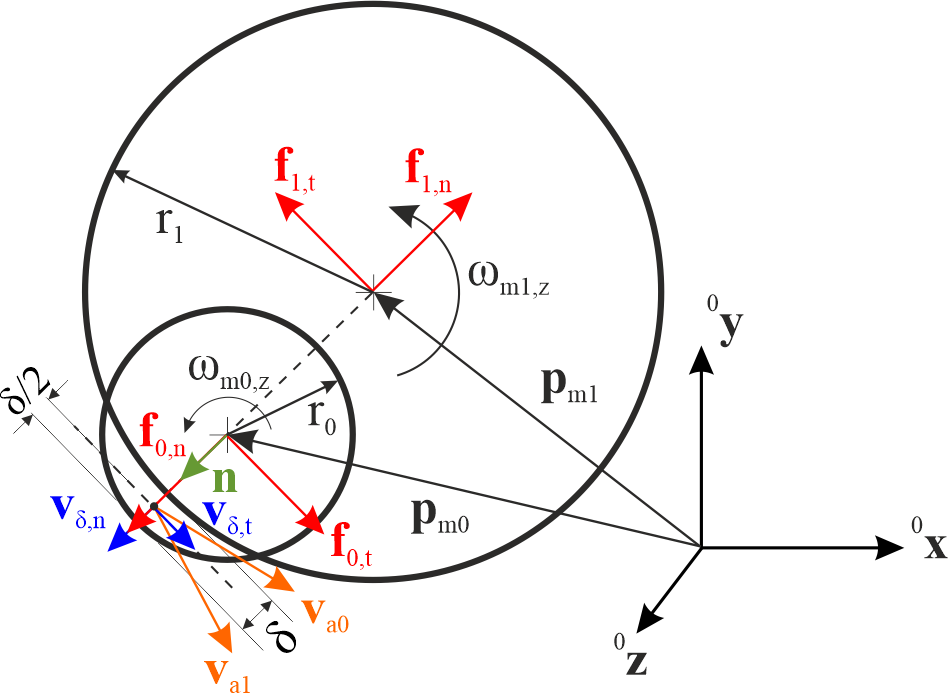
Fig. 44 One sphere and one hollowsphere that are in contact, showing a force on marker 1 against normal direction due to overlap; forces on marker 0 act in opposite direction.

To take the angular velocity of the spheres into account, the velocities \(\LU{0}{\vv}_{a0}\) and \(\LU{0}{\vv}_{a1}\) at the contact point are computed using Euler’s theorem for kinematics:

\[ \LU{0}{\vv}_{a0} = \LU{0}{\vv}_{m0} + \LU{0}{\tomega}_{m0} \times \left(\LU{0}{\nv}\cdot \left(r_0-\frac{\delta}{2}\right)\right) , \qquad \LU{0}{\vv}_{a1} = \LU{0}{\vv}_{m1} + h_1 \LU{0}{\tomega}_{m1} \times \left(-\LU{0}{\nv}\cdot \left(r_1-h_1 \frac{\delta}{2}\right)\right) \, . \]

For the velocity \(\LU{0}{\vv}_{a0}\) of sphere 0 at the contact point the sphere-sphere and sphere-hollowsphere contact cases are computed equally. For the velocity \(\LU{0}{\vv}_{a1}\) of sphere 1 at the contact point, one negative sign \(h_1\) is needed since the vector pointing to the contact point has the same direction for both spheres and one negative sign \(h_1\) is needed to correctly compute the length of the vector pointing from the center of sphere 1 to the contact point.

The normal force acting on marker 1 is generally written as

\[ \LU{0}{\fv}_\mathrm{1,n} = \underbrace{(f_c + f_d)}_{f_\mathrm{1,n}} \cdot \LU{0}{\nv} \, , \]

where \(f_c\) is the elastic and \(f_d\) the damping part. The damping \(f_d\) is always computed the same, independent of the chosen impact model:

\[ f_d = - d_c v_\mathrm{\delta,n} \, . \]

The negative sign is because of the damping acting against the gap velocity: in the case of a positive normal (gap) velocity, the damping acts against \(\LU{0}{\nv}\) for marker 1. As an illustrative case, the gap velocity is positive, if sphere 0 does not move, i.e. \(\LU{0}{\vv}_{m0}=0\) holds, and sphere 1 in direction of the normal vector. Note that this holds for the sphere-sphere contact and sphere-hollowsphere contact cases. The elastic force \(f_c\) is computed depending on the chosen impact model.

CASE \(m_\mathrm{impact}=0\): the Adhesive Elasto-Plastic model described in Morrissey2014 is used. This model captures the key bulk behavior of cohesive powders and granular soils. For the impact model, the plastic overlap \(\delta_p\) is needed. It is computed with

\[ \delta_p=\lambda_\mathrm{p}^{\frac{1}{n_\mathrm{exp}}}\delta \, . \]

The Adhesive Elasto-Plastic model distinguishes three different cases, modeling the loading and unloading behavior of the spheres:

\[\begin{split} f_c= \begin{cases} -f_\mathrm{adh} + k_c \delta^{n_\mathrm{exp}} & \text{if } k_2 \left(\delta^{n_\mathrm{exp}}-\delta_p^{n_\mathrm{exp}} \right) \geq k_c\delta^{n_\mathrm{exp}} \\ -f_\mathrm{adh} + k_2 \left(\delta^{n_\mathrm{exp}}-\delta_p^{n_\mathrm{exp}} \right) & \text{if } k_c\delta^{n_\mathrm{exp}} > k_2 \left(\delta^{n_\mathrm{exp}}-\delta_p^{n_\mathrm{exp}}\right) > -k_\mathrm{adh}\delta^{n_\mathrm{adh}} \\ -f_\mathrm{adh}-k_\mathrm{adh}\delta^{n_\mathrm{adh}} & \text{if } -k_\mathrm{adh}\delta^{n_\mathrm{adh}} > k_2 \left(\delta^{n_\mathrm{exp}}-\delta_p^{n_\mathrm{exp}} \right) \end{cases}\, . \end{split}\]

Note that \(k_2\) is computed with \(k_2 = k_c/(1-\lambda_\mathrm{P})\). The terms with the stiffness \(k_c\) and \(k_2\) have a positive sign, since they act in the direction of \(\LU{0}{\nv}\) for marker 1. The constant adhesion force \(f_\mathrm{adh}\) and the stiffness \(k_\mathrm{adh}\) act against \(\LU{0}{\nv}\), which corresponds to a force sticking the spheres together.

CASE \(m_\mathrm{impact}=1\): the restitution model proposed by Hunt and Crossley in Hunt1975 is used to simulate the energy loss of the spheres during contact:

\[ f_c=k_c \delta^{n_\mathrm{exp}} + \lambda \delta^{n_\mathrm{exp}} v_\mathrm{\delta,n} \]

with

\[ \lambda = \frac{k_c}{\dot\delta_\mathrm{-}}\frac{3}{2}(e_\mathrm{res}-1) \, . \]

The restitution coefficient \(e_\mathrm{res}\) describes the ration of the normal (gap) velocity before and after the impact of the spheres. In the case of \(e_\mathrm{res}<1\), the impact has a plastic portion, resulting in a force acting against \(\LU{0}{\nv}\) for marker 1, which is why \(\lambda\) must be negative in that case. \(\dot\delta_\mathrm{-}\) is the initial relative velocity, which is either the minimum impact velocity or the normal (negated gap) velocity:

\[ \dot\delta_\mathrm{-} = \max{\left(\dot\delta_\mathrm{-,min}; -v_\mathrm{\delta,n} \right)} \]

Note that the Hunt-Crossley restitution is valid for a very small energy loss (\(e_\mathrm{res}\approx1\)) Carvalho2019.

CASE \(m_\mathrm{impact}=2\): a generalization of the Hunt-Crossley restitution proposed by Carvalho and Martins in Carvalho2019 is used for \(e_\mathrm{res} > \frac{1}{3}\) and a model proposed by Gonthier et al. in Gonthier2004 is used for impacts with a high plastic proportion, \(e_\mathrm{res} < \frac{1}{3}\). Note that the two models are identical at \(e_\mathrm{res} = \frac{1}{3}\). \(\lambda\) is therefore computed as follows:

\[\begin{split} \lambda= \begin{cases} \frac{k_c}{\dot\delta_\mathrm{-}}\frac{3}{2}(e_\mathrm{res}-1)\frac{11-e_\mathrm{res}}{1+9e_\mathrm{res}} & \text{if } e_\mathrm{res} > \frac{1}{3} \\ \frac{k_c}{\dot\delta_\mathrm{-}}\frac{e_\mathrm{rep}^2-1}{e_\mathrm{rep}} & \text{if } e_\mathrm{res} > 0 \\ \end{cases}\, . \end{split}\]

The tangential force acting on marker 1 due to the friction model acts against the tangential velocity \(\vv_\mathrm{\delta,t}\), see the computation of \(\vv_\mathrm{\delta,t}\) in Equation (85). Thus, the tangential force for marker 1 is computed as

\[\begin{split} \LU{0}{\fv}_\mathrm{1,t} = -\LU{0}{\vv}_\mathrm{\delta,t} \cdot \begin{cases} \frac{\mu_d f_\mathrm{1,n}}{v_{reg}} & \text{if } v_{rel} < v_{reg} \\ \frac{\mu_d f_\mathrm{1,n}}{v_{rel}} & \text{else}\\ \end{cases} \, . \end{split}\]

Note that the case distinction above is made to ensure that for very small relative velocities the friction force does not become implausibly high. Taken together, the force acting on marker 1 due to the connector is computed as

\[ \LU{0}{\fv}_{m1}=\LU{0}{\fv}_\mathrm{1,n}+\LU{0}{\fv}_\mathrm{1,t} \, , \]

the force acting on marker 0 is \(\LU{0}{\fv}_{m0}=-\LU{0}{\fv}_{m1}\). The global torque \(\LU{0}{\ttau}_{m1}\) acting on marker 1 due to the connector is computed as

\[ \LU{0}{\ttau}_{m1}=-h_1 \LU{0}{\nv}\left( r_1-h_1 \frac{1}{2}\delta \right) \times \LU{0}{\fv}_{m1} \, , \]

and on marker 0 as

\[ \LU{0}{\ttau}_{m0}=\LU{0}{\nv} \left(r_0-\frac{1}{2}\delta \right) \times \LU{0}{\fv}_{m0}= \LU{0}{\nv}\left( r_0-\frac{1}{2}\delta \right) \times \left( -\LU{0}{\fv}_{m1} \right) \, . \]

It can be seen that the torque due to the connector is the same for both spheres, if \(r_0=r_1\) applies.

Mini example

#a ball dropped onto a large fixed sphere: penalty contact with its state in a data node
inertia = InertiaSphere(mass=1, radius=0.1)
node = mbs.AddNode(NodeRigidBodyEP(referenceCoordinates=[0,0,1.2]+eulerParameters0))
ball = mbs.AddObject(ObjectRigidBody(nodeNumber=node, mass=inertia.Mass(), inertia=inertia.GetInertia6D()))
mbs.AddLoad(LoadMassProportional(markerNumber=mbs.AddMarker(MarkerBodyMass(bodyNumber=ball)), loadVector=[0,0,-9.81]))
mGround = mbs.AddMarker(MarkerBodyRigid(bodyNumber=oGround, localPosition=[0,0,0]))
mBall = mbs.AddMarker(MarkerBodyRigid(bodyNumber=ball, localPosition=[0,0,0]))
nData = mbs.AddNode(NodeGenericData(numberOfDataCoordinates=4, initialCoordinates=[0,0,0,0]))
mbs.AddObject(ObjectContactSphereSphere(markerNumbers=[mGround, mBall], nodeNumber=nData, spheresRadii=[1, 0.1],
                                        contactStiffness=1e5, contactDamping=1e3))

mbs.Assemble()
simulationSettings = exu.SimulationSettings()
simulationSettings.timeIntegration.numberOfSteps = 1000
mbs.SolveDynamic(simulationSettings)

#at rest on top: 1.1 - m*g/k
exu.sys['testResult'] = mbs.GetNodeOutput(node, exu.OutputVariableType.Position)[2] #1.0999

Relevant Examples (Ex) and TestModels (TM) with weblink to github: newtonsCradle.py (Ex), rollerBearningModel.py (Ex), contactComparisonTest.py (TM), contactSphereSphereTest.py (TM), contactSphereSphereTestEAPM.py (TM), createSphereQuadContact.py (TM), createSphereTriangleContact.py (TM), explicitSolversPostNewtonTest.py (TM), inactiveConnectorForceTest.py (TM), sphereTriangleTest2.py (TM)