ObjectJointALEMoving2D

A specialized axially moving joint (without rotation) in 2D between a ALE Cable2D (marker1) and a position-based marker (marker0); ALE=Arbitrary Lagrangian Eulerian; the data coordinate x[0] provides the current index in slidingMarkerNumbers, and the ODE2 coordinate q[0] provides the (given) moving coordinate in the cable element.

Interface

Python names: ObjectJointALEMoving2D or ALEMovingJoint2D, and VALEMovingJoint2D for its visualization
Nodes: see the detailed description

Parameters

The parameters of the item; in a dictionary, its type is ‘JointALEMoving2D’:

name	type	default	description
name	String	‘’	constraints’s unique name
markerNumbers	ArrayMarkerIndex	[ invalid (-1), invalid (-1) ]	(symbol: \([m0,\,m1]\tp\)) marker m0: position-marker of mass point or rigid body; marker m1: updated marker to ANCF Cable2D element, where the sliding joint currently is attached to; must be initialized with an appropriate (global) marker number according to the starting position of the sliding object; this marker changes with time (PostNewtonStep)
slidingMarkerNumbers	ArrayMarkerIndex	[]	(symbol: \([m_{s0}, \ldots, m_{sn}]\tp\)) a list of sn (global) marker numbers which are are used to update marker1
slidingMarkerOffsets	Vector	[]	(symbol: \([d_{s0}, \ldots, d_{sn}]\)) this list contains the offsets of every sliding object (given by slidingMarkerNumbers) w.r.t. to the initial position (0): marker0: offset=0, marker1: offset=Length(cable0), marker2: offset=Length(cable0)+Length(cable1), …
slidingOffset	Real	0.	(symbol: \(s_\mathrm{off}\)) sliding offset [SI:m]: a scalar offset, which represents the (reference arc) length of all previous sliding cable elements
nodeNumbers	ArrayNodeIndex	[ invalid (-1), invalid (-1) ]	(symbol: \([n_{GD}, n_{ALE}]\)) node number of NodeGenericData (GD) with one data coordinate and of NodeGenericODE2 (ALE) with one ODE2 coordinate
usePenaltyFormulation	Bool	False	flag, which determines, if the connector is formulated with penalty, but still using algebraic equations (IsPenaltyConnector() still false)
penaltyStiffness	Real	0.	(symbol: \(k\)) penalty stiffness [SI:N/m] used if usePenaltyFormulation=True
activeConnector	Bool	True	flag, which determines, if the connector is active; used to deactivate (temporarily) a connector or constraint
visualization	VObjectJointALEMoving2D		parameters for visualization of item

Visualization parameters

The parameters of VObjectJointALEMoving2D, given as visualization:

name	type	size	default	description
show	Bool		True	set true, if item is shown in visualization and false if it is not shown
drawSize	float		-1.	drawing size = radius of revolute joint; size == -1.f means that default connector size is used
color	Float4	4	[-1.,-1.,-1.,-1.]	RGBA connector color; if R==-1, use default color

Drawing

Drawn as all joints; a circle of diameter drawSize at marker 0 and at the sliding position, with a cross there.

Output variables

Available as OutputVariableType in sensors, Get...Output() and other functions:

output variable	symbol	description
Position	\(\LU{0}{\pv}_{m0}\)	current global position of position marker \(m0\)
Velocity	\(\LU{0}{\vv}_{m0}\)	current global velocity of position marker \(m0\)
SlidingCoordinate	\(s_g = q_{ALE} + s_\mathrm{off}\)	current value of the global sliding ALE coordinate, including offset; note that reference coordinate of \(q_{ALE}\) is ignored!
Coordinates	\([x_{data0},\,q_{ALE}]\tp\)	provides two values: [0] = current sliding marker index, [1] = ALE sliding coordinate
Coordinates_t	\([\dot q_{ALE}]\tp\)	provides ALE sliding velocity
Force	\(\fv\)	joint force vector (3D)

Detailed description

Definition of quantities

intermediate variables	symbol	description
generic data node	\(\xv=[x_{data0}]\tp\)	coordinates of node with node number \(n_{GD}\)
generic ODE2 node	\(\qv=[q_{0}]\tp\)	coordinates of node with node number \(n_{ALE}\), which is shared with all ALE-ANCF and ALE sliding joint objects
data coordinate	\(x_{data0}\)	the current index in slidingMarkerNumbers
ALE coordinate	\(q_{ALE} = q_{0}\)	current ALE coordinate (in fact this is the Eulerian coordinate in the ALE formulation); note that reference coordinate of \(q_{ALE}\) is ignored!
marker m0 position	\(\LU{0}{\pv}_{m0}\)	current global position which is provided by marker m0
marker m0 velocity	\(\LU{0}{\vv}_{m0}\)	current global velocity which is provided by marker m0
cable coordinates	\(\qv_{ANCF,m1}\)	current coordiantes of the ANCF cable element with the current marker \(m1\) is referring to
sliding position	\(\LUR{0}{\rv}{ANCF} = \Sm(s_{el})\qv_{ANCF,m1}\)	current global position at the ANCF cable element, evaluated at local sliding position \(s_{el}\)
sliding position slope	\(\LURU{0}{\rv}{ANCF}{\prime} = \Sm^\prime(s_{el})\qv_{ANCF,m1}\)	current global slope vector of the ANCF cable element, evaluated at local sliding position \(s_{el}\)
sliding velocity	\(\LUR{0}{\vv}{ANCF} = \Sm(s_{el})\dot\qv_{ANCF,m1} + \dot q_{ALE} \LURU{0}{\rv}{ANCF}{\prime}\)	current global velocity at the ANCF cable element, evaluated at local sliding position \(s_{el}\), including convective term
sliding normal vector	\(\LU{0}{\nv} = [-r^\prime_1,\,r^\prime_0]\)	2D normal vector computed from slope \(\rv^\prime=\LURU{0}{\rv}{ANCF}{\prime}\)
algebraic variables	\(\zv=[\lambda_0,\,\lambda_1]\tp\)	algebraic variables (Lagrange multipliers) according to the algebraic equations

Geometric relations

The element sliding coordinate (in the local coordinates of the current sliding element) is computed from the ALE coordinate

\[ s_{el} = q_{ALE} + s_\mathrm{off} - d_{m1} = s_g - d_{m1}. \]

For the description of the according quantities, see the description above. The distance \(d_{m1}\) is obtained from the slidingMarkerOffsets list, using the current (local) index \(x_{data0}\). The vector (=difference; error) between the marker \(m0\) and the marker \(m1\) (=\(\rv_{ANCF}\)) positions reads

\[ \LU{0}{\Delta\pv} = \LUR{0}{\rv}{ANCF} - \LU{0}{\pv}_{m0} \]

Note that \(\LU{0}{\pv}_{m0}\) represents the current position of the marker \(m0\), which could represent the midpoint of a mass sliding along the beam. The position \(\LUR{0}{\rv}{ANCF}\) is computed from the beam represented by marker \(m1\), using the local beam coordinate \(x=s_{el}\). The marker and the according beam finite element changes during movement using the list slidingMarkerNumbers and the index is updated in the PostNewtonStep. The vector (=difference; error) between the marker \(m0\) and the marker \(m1\) velocities reads

\[ \LU{0}{\Delta\vv} = \LUR{0}{\vv}{ANCF} - \LU{0}{\vv}_{m0} \]

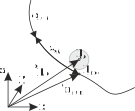
../../../_images/ObjectJointALEmoving2D.svg — Fig. 45 Geometrical relations for ALE sliding joint.

Connector constraint equations

The 2D sliding joint is implemented having 2 equations, using the Lagrange multipliers \(\zv\). The algebraic (index 3) equations read

\[ \LU{0}{\Delta\pv} = 0 \]

Note that the Lagrange multipliers \([\lambda_0,\,\lambda_1]\tp\)are the global forces in the joint. In the index 2 case the algebraic equations read

\[ \LU{0}{\Delta\vv} = 0 \]

If usePenalty = True, the algebraic equations are changed to:

\[ \LU{0}{\Delta \pv} - \frac 1 k \zv = 0. \]

If activeConnector = False, the algebraic equations are changed to:

\[\begin{split} \begin{aligned} \lambda_0 &= 0, \\ \lambda_1 &= 0. \end{aligned} \end{split}\]

Post Newton Step

After the Newton solver has converged, a PostNewtonStep is performed for the element, which updates the marker \(m1\) index if necessary.

\[\begin{split} \begin{aligned} s_{el} < 0 \quad \ra \quad x_{data0} \;-\!\!=1 \\ s_{el} > L \quad \ra \quad x_{data0} \;+\!\!=1 \end{aligned} \end{split}\]

Furthermore, it is checked, if \(x_{data0}\) becomes smaller than zero, which raises a warning and keeps \(x_{data0}=0\). The same results if \(x_{data0}\ge sn\), then \(x_{data0} = sn\). Finally, the data coordinate is updated in order to provide the starting value for the next step,

\[ x_{data1} \;+\!\!= s. \]

Mini example

from exudyn.beams import GenerateBeamElementsAlongLine
#a mass point carried by the material of an axially moving cable
nALE = mbs.AddNode(NodeGenericODE2(numberOfODE2Coordinates=1, referenceCoordinates=[0],
                                   initialCoordinates=[0], initialCoordinates_t=[0]))
cable = ObjectALEANCFCable2D(massPerLength=1, bendingStiffness=10, axialStiffness=1e4)
cable.nodeNumbers[2] = nALE
beamInfo = GenerateBeamElementsAlongLine(mbs, positionStart=[0,0,0], positionEnd=[2,0,0],
                        numberOfElements=4, beamTemplate=cable,
                        groundConstraintsStart=[1,1,1,1], groundConstraintsEnd=[1,1,1,1])
nodes, elements = beamInfo['nodes'], beamInfo['elements']
mbs.AddLoad(LoadCoordinate(markerNumber=mbs.AddMarker(MarkerNodeCoordinate(nodeNumber=nALE, coordinate=0)), load=1))

nMass = mbs.AddNode(NodePoint2D(referenceCoordinates=[0.6,0]))
mbs.AddObject(ObjectMassPoint2D(nodeNumber=nMass, mass=2))
cableMarkers = [mbs.AddMarker(MarkerBodyCable2DCoordinates(bodyNumber=e)) for e in elements]
nData = mbs.AddNode(NodeGenericData(numberOfDataCoordinates=1, initialCoordinates=[1])) #element 1
mbs.AddObject(ObjectJointALEMoving2D(markerNumbers=[mbs.AddMarker(MarkerNodePosition(nodeNumber=nMass)), cableMarkers[1]],
                                     slidingMarkerNumbers=cableMarkers, slidingMarkerOffsets=[0.5*i for i in range(4)],
                                     slidingOffset=0.6, nodeNumbers=[nData, nALE]))

mbs.Assemble()
mbs.SolveDynamic()

#cable material (mass 2) and mass point (2) move together: x = 0.6 + F/(2*4)*t^2 at t=1
exu.sys['testResult'] = mbs.GetNodeOutput(nMass, exu.OutputVariableType.Position)[0] #0.725

Relevant Examples (Ex) and TestModels (TM) with weblink to github: ANCFmovingRigidbody.py (Ex), ANCFmovingRigidBodyTest.py (TM)