ObjectJointSliding2D

A specialized sliding joint (without rotation) in 2D between a Cable2D (marker1) and a position-based marker (marker0); the data coordinate x[0] provides the current index in slidingMarkerNumbers, and x[1] the local position in the cable element at the beginning of the timestep.

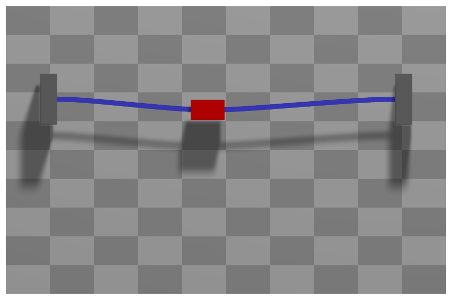
Interface

Python names: ObjectJointSliding2D or SlidingJoint2D, and VSlidingJoint2D for its visualization
Nodes it takes: NodeGenericData

Parameters

The parameters of the item; in a dictionary, its type is ‘JointSliding2D’:

name	type	default	description
name	String	‘’	constraints’s unique name
markerNumbers	ArrayMarkerIndex	[ invalid (-1), invalid (-1) ]	(symbol: $[m0,m1]\tp$) marker m0: position or rigid body marker of mass point or rigid body; marker m1: updated marker to Cable2D element, where the sliding joint currently is attached to; must be initialized with an appropriate (global) marker number according to the starting position of the sliding object; this marker changes with time (PostNewtonStep)
slidingMarkerNumbers	ArrayMarkerIndex	[]	(symbol: $[m_{s0}, \ldots, m_{sn}]\tp$) these markers are used to update marker m1, if the sliding position exceeds the current cable’s range; the markers must be sorted such that marker $m_{si}$ at x=cable(i).length is equal to marker(i+1) at x=0 of cable(i+1)
slidingMarkerOffsets	Vector	[]	(symbol: $[d_{s0}, \ldots, d_{sn}]$) this list contains the offsets of every sliding object (given by slidingMarkerNumbers) w.r.t. to the initial position (0): marker m0: offset=0, marker m1: offset=Length(cable0), marker m2: offset=Length(cable0)+Length(cable1), …
nodeNumber	NodeIndex	invalid (-1)	(symbol: $n_{GD}$) node number of a NodeGenericData for 1 dataCoordinate showing the according marker number which is currently active and the start-of-step (global) sliding position
useClassicalFormulation	Bool	True	True: uses a formulation with 3 (+1) equations, including the force in sliding direction to be zero; forces in global coordinates, only index 3; False: use local formulation, which only needs 2 (+1) equations and can be used with index 2 formulation
constrainRotation	Bool	False	True: add constraint on rotation of marker m0 relative to slope (if True, marker m0 must be a rigid body marker); False: marker m0 body can rotate freely
axialForce	Real	0	(symbol: $f_\mathrm{ax}$) ONLY APPLIES if useClassicalFormulation==True; axialForce represents an additional sliding force acting between beam and marker m0 body in axial (beam) direction; this force can be used to drive a body on a beam, but can only be changed with user functions.
activeConnector	Bool	True	flag, which determines, if the connector is active; used to deactivate (temporarily) a connector or constraint
visualization	VObjectJointSliding2D		parameters for visualization of item

Renamed parameters, still taken with a DeprecationWarning: classicalFormulation (deprecated since 1.12.258, removed in 2031): use useClassicalFormulation.

Visualization parameters

The parameters of VObjectJointSliding2D, given as visualization:

name	type	size	default	description
show	Bool		True	set true, if item is shown in visualization and false if it is not shown
drawSize	float		-1.	drawing size = radius of revolute joint; size == -1.f means that default connector size is used
color	Float4	4	[-1.,-1.,-1.,-1.]	RGBA connector color; if R==-1, use default color

Drawing

Drawn as all joints; a circle of diameter drawSize at each marker, the one of marker 0 red.

Output variables

Available as OutputVariableType in sensors, Get...Output() and other functions:

output variable	symbol	description
Position		position vector of joint given by marker0
Velocity		velocity vector of joint given by marker0
SlidingCoordinate		global sliding coordinate along all elements; the maximum sliding coordinate is equivalent to the reference lengths of all sliding elements
Force		joint force vector (3D)
DisplacementLocal	$[\Delta\pv\tp\tv,\;\Delta\pv\tp\nv,\;0]\tp$	position of the sliding point on the cable relative to marker m0, $\Delta\pv$, along the unit tangent $\tv$ and the unit normal $\nv$ of the cable there: the drift of the joint

Detailed description

Definition of quantities

intermediate variables	symbol	description
data node	$\xv=[x_{data0},\,x_{data1}]\tp$	coordinates of node with node number $n_{GD}$
data coordinate 0	$x_{data0}$	the current index in slidingMarkerNumbers
data coordinate 1	$x_{data1}$	the global sliding coordinate (ranging from 0 to the total length of all sliding elements) at start-of-step - beginning of the timestep
marker m0 position	$\LU{0}{\pv}_{m0}$	current global position which is provided by marker m0
marker m0 velocity	$\LU{0}{\vv}_{m0}$	current global velocity which is provided by marker m0
marker m0 orientation	$\LU{0,m0}{\Rot}$	current rotation matrix provided by marker m0 (assumed to be rigid body)
marker m0 angular velocity	$\LU{0}{\tomega}_{m0}$	current angular velocity vector provided by marker m0 (assumed to be rigid body)
cable coordinates	$\qv_{ANCF,m1}$	current coordiantes of the ANCF cable element with the current marker $m1$ is referring to
sliding position	$\LUR{0}{\rv}{ANCF} = \Sm(s_{el})\qv_{ANCF,m1}$	current global position at the ANCF cable element, evaluated at local sliding position $s_{el}$
sliding position slope	$\LURU{0}{\rv}{ANCF}{\prime} = \Sm^\prime(s_{el})\qv_{ANCF,m1} = [r^\prime_0,\,r^\prime_1]\tp$	current global slope vector of the ANCF cable element, evaluated at local sliding position $s_{el}$
sliding velocity	$\LUR{0}{\vv}{ANCF} = \Sm(s_{el})\dot\qv_{ANCF,m1}$	current global velocity at the ANCF cable element, evaluated at local sliding position $s_{el}$ ($s_{el}$ not differentiated!!!)
sliding velocity slope	$\LURU{0}{\vv}{ANCF}{\prime} = \Sm^\prime(s_{el})\dot\qv_{ANCF,m1}$	current global slope velocity vector of the ANCF cable element, evaluated at local sliding position $s_{el}$
sliding normal vector	$\LU{0}{\nv} = [-r^\prime_1,\,r^\prime_0]$	2D normal vector computed from slope $\rv^\prime=\LURU{0}{\rv}{ANCF}{\prime}$
sliding normal velocity vector	$\LU{0}{\dot\nv} = [-\dot r^\prime_1,\,\dot r^\prime_0]$	time derivative of 2D normal vector computed from slope velocity $\dot \rv^\prime=\LURU{0}{\dot \rv}{ANCF}{\prime}$
algebraic coordinates	$\zv=[\lambda_0,\,\lambda_1,\, s]\tp$	algebraic coordinates composed of Lagrange multipliers $\lambda_0$ and $\lambda_1$ (in local cable coordinates: $\lambda_0$ is in axis direction) and the current sliding coordinate $s$, which is local in the current cable element.
local sliding coordinate	$s$	local incremental sliding coordinate $s$: the (algebraic) sliding coordinate relative to the start-of-step value. Thus, $s$ only contains small local increments.

output variables	symbol	formula
Position	$\LU{0}{\pv}_{m0}$	current global position of position marker $m0$
Velocity	$\LU{0}{\vv}_{m0}$	current global velocity of position marker $m0$
SlidingCoordinate	$s_g = s + x_{data1}$	current value of the global sliding coordinate
Force	$\fv$	see below

Geometric relations

Assume we have given the sliding coordinate $s$ (e.g., as a guess of the Newton method or beginning of the time step). The element sliding coordinate (in the local coordinates of the current sliding element) is computed as

\[ s_{el} = s + x_{data1} - d_{m1} = s_g - d_{m1}. \]

The vector (=difference; error) between the marker $m0$ and the marker $m1$ (=$\rv_{ANCF}$) positions reads

\[ \LU{0}{\Delta\pv} = \LUR{0}{\rv}{ANCF} - \LU{0}{\pv}_{m0} \]

The vector (=difference; error) between the marker $m0$ and the marker $m1$ velocities reads

\[ \LU{0}{\Delta\vv} = \LUR{0}{\dot\rv}{ANCF} - \LU{0}{\vv}_{m0} \]

Connector constraint equations (useClassicalFormulation=True)

The 2D sliding joint is implemented having 3 equations (4 if constrainRotation==True, see below), using the special algebraic coordinates $\zv$. The algebraic equations read

\[\begin{split} \begin{aligned} \LU{0}{\Delta\pv} &= \Null, \quad \mbox{... two index 3 eqs $\ra$ sliding body stays on cable}\\ \left[\lambda_0,\lambda_1\right] \cdot \LURU{0}{\rv}{ANCF}{\prime} - |\LURU{0}{\rv}{ANCF}{\prime}| \cdot f_\mathrm{ax} &= 0, \quad \mbox{... one index 1 equ. $\ra$ force in sliding dir.=$f_\mathrm{ax}$} \\ \end{aligned} \end{split}\]

No index 2 case exists, because no time derivative exists for $s_{el}$. The jacobian matrices for algebraic and ODE2 coordinates read

\[ \Jm_{AE} = \mr{0}{0}{r^\prime_0} {0}{0}{r^\prime_1} {r^\prime_0}{r^\prime_1}{r^{\prime\prime}_0\lambda_0 + r^{\prime\prime}_1\lambda_1} \]

\[ \Jm_{ODE2} = \mp{-J_{pos,m0}}{\Sm(s_{el})} {\Null\tp}{\left[\lambda_0,\,\lambda_1\right]\cdot\Sm^\prime(s_{el}) } \]

if activeConnector = False, the algebraic equations are changed to:

\[\begin{split} \begin{aligned} \lambda_0 &= 0, \\ \lambda_1 &= 0, \\ s &= 0 \end{aligned} \end{split}\]

Connector constraint equations (useClassicalFormulation=False)

The 2D sliding joint is implemented having 3 equations (first equation is dummy and could be eliminated; 4 equations if constrainRotation==True, see below), using the special algebraic coordinates $\zv$. The algebraic equations read

\[\begin{split} \begin{aligned} \lambda_0 &= 0, \quad \mbox{... eq.~not necessary, but can be used for switching to other modes} \\ \LU{0}{\Delta\pv\tp} \LU{0}{\nv} &= 0, \quad \mbox{... eq.~ensures that sliding body stays at cable centerline; index3}\\ \LU{0}{\Delta\pv\tp} \LURU{0}{\rv}{ANCF}{\prime} &= 0. \quad \mbox{... resolves the sliding coordinate $s$; index1 eq.!} \end{aligned} \end{split}\]

In the index 2 case, the second equation reads

\[ \LU{0}{\Delta\vv\tp} \LU{0}{\nv} + \LU{0}{\Delta\pv\tp} \LU{0}{\dot\nv} = 0 \, . \]

If activeConnector = False, the algebraic equations are changed to:

\[\begin{split} \begin{aligned} \lambda_0 &= 0, \\ \lambda_1 &= 0, \\ s &= 0 \end{aligned} \end{split}\]

In case that constrainRotation = True, an additional constraint is added for the relative rotation between the slope of the cable and the orientation of marker m0 body. Assuming that the orientation of marker m0 is a 2D matrix (taking only $x$ and $y$ coordinates), the constraint reads

\[ \LURU{0}{\rv}{ANCF}{\prime\mathrm{T}} \LU{0,m0}{\Rot} \vp{0}{1} = 0 \]

The index 2 case follows straightforward to

\[ \LURU{0}{\dot \rv}{ANCF}{\prime\mathrm{T}} \LU{0,m0}{\Rot} \vp{0}{1} + \LURU{0}{\rv}{ANCF}{\prime\mathrm{T}} \LU{0,m0}{\Rot} \LU{0}{\tilde \tomega}_{m0} \vp{0}{1} = 0 \]

again assuming, that $\LU{0}{\tilde \tomega}_{m0}$ is only a $2 \times 2$ matrix.

Post Newton Step

After the Newton solver has converged, a PostNewtonStep is performed for the element, which updates the marker $m1$ index if necessary.

\[\begin{split} \begin{aligned} s_{el} < 0 \quad \ra \quad x_{data0}\;-\!\!=1 \\ s_{el} > L \quad \ra \quad x_{data0}\;+\!\!=1 \end{aligned} \end{split}\]

Furthermore, it is checked, if $x_{data0}$ becomes smaller than zero, which raises a warning and keeps $x_{data0}=0$. The same results if $x_{data0}\ge sn$, then $x_{data0} = sn$. Finally, the data coordinate is updated in order to provide the starting value for the next step,

\[ x_{data1} \;+\!\!= s. \]

Mini example

from exudyn.beams import GenerateBeamElementsAlongLine
#the coordinates of ANCF cable elements for a sliding joint: a mass point slides along a clamped, stiff cable
cable = ObjectANCFCable2D(massPerLength=1, bendingStiffness=1e4, axialStiffness=1e6)
beamInfo = GenerateBeamElementsAlongLine(mbs, positionStart=[0,0,0], positionEnd=[2,0,0],
                        numberOfElements=4, beamTemplate=cable,
                        groundConstraintsStart=[1,1,1,1], groundConstraintsEnd=[1,1,1,1])
nodes, elements = beamInfo['nodes'], beamInfo['elements']
nMass = mbs.AddNode(NodePoint2D(referenceCoordinates=[0.6,0]))
mbs.AddObject(ObjectMassPoint2D(nodeNumber=nMass, mass=1))
mMass = mbs.AddMarker(MarkerNodePosition(nodeNumber=nMass))
mbs.AddLoad(LoadForceVector(markerNumber=mMass, loadVector=[1,0,0]))

cableMarkers = [mbs.AddMarker(MarkerBodyCable2DCoordinates(bodyNumber=e)) for e in elements]
offsets = [0.5*i for i in range(4)] #the element length is 0.5
nData = mbs.AddNode(NodeGenericData(numberOfDataCoordinates=2, initialCoordinates=[1, 0.6])) #element 1, sliding coordinate
mbs.AddObject(ObjectJointSliding2D(markerNumbers=[mMass, cableMarkers[1]], slidingMarkerNumbers=cableMarkers,
                                   slidingMarkerOffsets=offsets, nodeNumber=nData))

mbs.Assemble()
mbs.SolveDynamic()

#the mass slides: x = 0.6 + F/(2m)*t^2 at t=1, the stiff cable deflects little
exu.sys['testResult'] = mbs.GetNodeOutput(nMass, exu.OutputVariableType.Position)[0] #1.1

Relevant Examples (Ex) and TestModels (TM) with weblink to github: ANCFmovingRigidbody.py (Ex), ANCFslidingJoint2D.py (Ex), ANCFslidingJoint2Drigid.py (Ex), ANCFswitchingSlidingJoint2D.py (Ex), SlidingJoint2DTest.py (TM)

intermediate variables	symbol	description
data node	\(\xv=[x_{data0},\,x_{data1}]\tp\)	coordinates of node with node number \(n_{GD}\)
data coordinate 0	\(x_{data0}\)	the current index in slidingMarkerNumbers
data coordinate 1	\(x_{data1}\)	the global sliding coordinate (ranging from 0 to the total length of all sliding elements) at start-of-step - beginning of the timestep
marker m0 position	\(\LU{0}{\pv}_{m0}\)	current global position which is provided by marker m0
marker m0 velocity	\(\LU{0}{\vv}_{m0}\)	current global velocity which is provided by marker m0
marker m0 orientation	\(\LU{0,m0}{\Rot}\)	current rotation matrix provided by marker m0 (assumed to be rigid body)
marker m0 angular velocity	\(\LU{0}{\tomega}_{m0}\)	current angular velocity vector provided by marker m0 (assumed to be rigid body)
cable coordinates	\(\qv_{ANCF,m1}\)	current coordiantes of the ANCF cable element with the current marker \(m1\) is referring to
sliding position	\(\LUR{0}{\rv}{ANCF} = \Sm(s_{el})\qv_{ANCF,m1}\)	current global position at the ANCF cable element, evaluated at local sliding position \(s_{el}\)
sliding position slope	\(\LURU{0}{\rv}{ANCF}{\prime} = \Sm^\prime(s_{el})\qv_{ANCF,m1} = [r^\prime_0,\,r^\prime_1]\tp\)	current global slope vector of the ANCF cable element, evaluated at local sliding position \(s_{el}\)
sliding velocity	\(\LUR{0}{\vv}{ANCF} = \Sm(s_{el})\dot\qv_{ANCF,m1}\)	current global velocity at the ANCF cable element, evaluated at local sliding position \(s_{el}\) (\(s_{el}\) not differentiated!!!)
sliding velocity slope	\(\LURU{0}{\vv}{ANCF}{\prime} = \Sm^\prime(s_{el})\dot\qv_{ANCF,m1}\)	current global slope velocity vector of the ANCF cable element, evaluated at local sliding position \(s_{el}\)
sliding normal vector	\(\LU{0}{\nv} = [-r^\prime_1,\,r^\prime_0]\)	2D normal vector computed from slope \(\rv^\prime=\LURU{0}{\rv}{ANCF}{\prime}\)
sliding normal velocity vector	\(\LU{0}{\dot\nv} = [-\dot r^\prime_1,\,\dot r^\prime_0]\)	time derivative of 2D normal vector computed from slope velocity \(\dot \rv^\prime=\LURU{0}{\dot \rv}{ANCF}{\prime}\)
algebraic coordinates	\(\zv=[\lambda_0,\,\lambda_1,\, s]\tp\)	algebraic coordinates composed of Lagrange multipliers \(\lambda_0\) and \(\lambda_1\) (in local cable coordinates: \(\lambda_0\) is in axis direction) and the current sliding coordinate \(s\), which is local in the current cable element.
local sliding coordinate	\(s\)	local incremental sliding coordinate \(s\): the (algebraic) sliding coordinate relative to the start-of-step value. Thus, \(s\) only contains small local increments.